| Partial differential equations |
In engineering sciences, partial differential equations play an important and central role. For example, the temperature of a metal plate can be expressed as a partial differential equation if the temperature on the boundaries is known. This is called a boundary value problem.
Usually, it is not easy to solve these problems. Analytical solutions exist only in very special cases. But there are some more or less "good" numerical ways to solve boundary value problems.
We now will look at one method which works with finite difference
approximations for the derivatives of a function. For this approach, we do not
look at an analytical function u(x) but we are only interested in
the values of u at a finite set of discrete points ![]() .
The distance between two adjacent points,
.
The distance between two adjacent points, ![]() and
and
![]() , is constant:
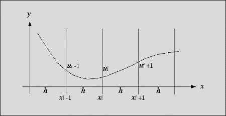
, is constant: ![]() (cf. figure 1).
(cf. figure 1).

Figure: u(x) at
some discrete points ![]()
The finite difference approximation of a first derivative of the function u(x) is
![]()
The second derivative is approximated by
![]()
This approximation works with 2-dimensional functions
u(x,y) as well. For simplicity we only work on square
problems, i.e. (x, y) is element of ![]() .
Again, the area of the function is discretized in a similar way:
.
Again, the area of the function is discretized in a similar way: ![]() , for some integer
, for some integer ![]() . We only look at the values of
u(x,y) at the discrete points
. We only look at the values of
u(x,y) at the discrete points ![]() .
With this discretization, we have a function
.
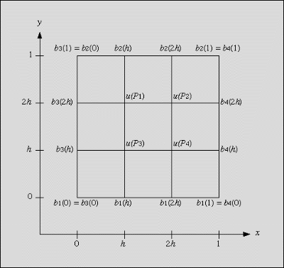
With this discretization, we have a function ![]() as
shown in figure 2:
as
shown in figure 2:

Figure: Function ![]() in the discretization area
in the discretization area
On the boundary, ![]() is given by 4 known functions:
is given by 4 known functions:

The points ![]() cover the inner points of the
discretization area, i.e. the area without the boundary. They are numbered from
left to right and from top to bottom like English text.
cover the inner points of the
discretization area, i.e. the area without the boundary. They are numbered from
left to right and from top to bottom like English text.
What we now want to do is to solve the poisson-equation in the area ![]() :
:
![]()
with the above boundary conditions. f(x,y) is a given 2-dimensional function. With equation (2) and the above discretization, the poisson-equation can be approximated at
![]()
where ![]() is the function
f(x,y), evaluated at the discrete points
is the function
f(x,y), evaluated at the discrete points ![]() .
.
Formula (5) can be written in a more readable form, depending on the position of the discrete points:

A similar equation, which we will use as an example below, is:

We call the ![]() matrix on the left hand side v and
the
matrix on the left hand side v and
the ![]() matrix on the right hand side g.
matrix on the right hand side g.
Now, equation (6b) can be formulated in every point of the discrete area of figure 2:

and (7) is a linear equation system for the values of
u(x,y) at the points ![]() and
and
![]() .
.
By rearranging and adding the terms on each line, the linear equation system can be formulated as:
![]()
where a is a ![]() matrix and b is a vector with 4
elements. Vector z represents the unknown values of
u(x,y) at the points
matrix and b is a vector with 4
elements. Vector z represents the unknown values of
u(x,y) at the points ![]() and
and
![]() .
.
You are to write a program that creates the linear equation system (7) in the
form (8) for any two matrices v and g (6). As input, the two
matrices v and g and the functions ![]() ,
and f are given. Also, a parameter n is given as the number of
discretization intervals. Thus,
,
and f are given. Also, a parameter n is given as the number of
discretization intervals. Thus, ![]() . As the result, your program
should calculate the matrix a and the vector b. For this more
general case, there are
. As the result, your program
should calculate the matrix a and the vector b. For this more
general case, there are ![]() inner points and a and b
must be sized accordingly.
inner points and a and b
must be sized accordingly.
The input file consists of m tests. The number m is given in
the first line of the file. The first line of each test contains the number
n which gives the number of discretizations intervals as defined above.
You may assume that ![]() . Then the
. Then the ![]() matrices v and g follow. The following four lines contain the
functions
matrices v and g follow. The following four lines contain the
functions ![]() and
and ![]() ,
each given as a vector of order n+1, containing the values for 0,
h, 2h, ..., 1. Finally, the function f is given as a
n+1 by n+1 matrix. Like the vectors before, it contains the values
for
,
each given as a vector of order n+1, containing the values for 0,
h, 2h, ..., 1. Finally, the function f is given as a
n+1 by n+1 matrix. Like the vectors before, it contains the values
for ![]() . Each row contains from left to right
the function values for increasing x values while each column contains
from top to bottom the function values for increasing y values.
. Each row contains from left to right
the function values for increasing x values while each column contains
from top to bottom the function values for increasing y values.
A vector occupies one line. Its values are given in ascending order, separated by a space. A n by n matrix occupies n lines. Its rows are given in ascending order as vectors, which occupy one line each. All values found in the input file are integer values.
For each test found in the input file, your program should output the
matrices a and b. Matrix a is a ![]() matrix (the discretization area (cf. figure 2) contains
matrix (the discretization area (cf. figure 2) contains ![]() inner points, which are unknown). The vector b is of order
inner points, which are unknown). The vector b is of order ![]() . They should be output in the same format as the vectors and matrices
in the input file. Your output should only contain integer values. Note that the
expression
. They should be output in the same format as the vectors and matrices
in the input file. Your output should only contain integer values. Note that the
expression ![]() yields an integer number and that all
other calculations can also be done using integer numbers.
yields an integer number and that all
other calculations can also be done using integer numbers.
1
3
1 0 2
0 -4 0
3 0 4
0 5 0
6 0 7
0 8 0
3 4 5 6
0 1 2 3
3 2 1 0
6 5 4 3
1 1 1 1
2 2 2 2
3 3 3 3
4 4 4 4
-36 0 0 36
0 -36 27 0
0 18 -36 0
9 0 0 -36
-8 -152 -198 -333